

In this post: avoiding some issues when mapping from rotations to unitary matrices, and running into different issues.
Common Mapping
Last week I mentioned (and relied on the fact) that the space of 2x2 unitary matrices is very similar to the space of rotations. More specifically, 2x2 unitary matrices are isomorphic to the biquaternions (i.e. the complexification of the quaternions, because the quaternions weren't complex enough I guess).
Given that unitary matrices are "like" rotations, a thing you might occasionally want to do is convert a rotation into some unitary matrix that corresponds to the rotation in some useful way. The easiest way to do this, and the one you'll find if you go looking, is to represent the rotation as a quaternion and then replace the quaternion components with corresponding Pauli matrices times $i$:
$1 \rightarrow I = \begin{bmatrix} 1 & 0 \\ 0 & 1 \end{bmatrix}$
$i \rightarrow i \: \sigma_x = \begin{bmatrix} 0 & i \\ i & 0 \end{bmatrix}$
$j \rightarrow i \: \sigma_y = \begin{bmatrix} 0 & 1 \\ -1 & 0 \end{bmatrix}$
$k \rightarrow i \: \sigma_z = \begin{bmatrix} i & 0 \\ 0 & -i \end{bmatrix}$
If our input rotation is a vector $v$, where the direction of $v$ is the rotation axis and the length $|v|$ is how much to rotate in radians, then the unitary matrix we will convert that rotation into is:
$U(v) = I \cos{\frac{|v|}{2}} + i \hat{v} \sigma_{xyz} \sin{\frac{|v|}{2}}$
Where $\hat{v} \sigma_{xyz}$ gives you the Pauli vector along $v$.
Flaws
The common mapping has a lot of nice properties, but has two flaws I would like to avoid.
The first flaw is that the angles are being divided by two. Because of that, a 360° turn doesn't get you back to where you started: it gets you to $-I$. If we use this mapping, then we'd have to "turn" 720° to really get back to the starting point. That's kind of confusing.
The second flaw is that there's no rotation corresponding to the Pauli matrices. A 180° turn around the X axis gives us $i \sigma_x$ instead of just $\sigma_x$. That means that, if we wanted to use these rotations to define operations for a quantum computer, we can't even make a NOT gate! (At least, not without an annoying global phase factor tacked on.)
Is it possible to avoid those flaws? Yes, but it will cost us something else.
Phase Correction
Both flaws I mentioned are caused by one problem: the global phase factor is wrong. What we need to do is add a specially crafted counter-phase factor.
Currently a half-turn around the X axis gives us $i \sigma_x$. To turn it into $\sigma_x$ we'll need a phase correction factor of $-i$. Similarly, we'll want a phase correction factor of $-1$ for one full turn. Also, after three half turns around the X axis (or one half turn around the negative X axis), we want a phase correction factor of $i$. The phase correction factors are the same for the Y and Z axies, with respect to the amount of turning.
Given the above information, it's clear we need a correction factor like $e ^{i s \frac{|v|}{2}}$ where $s$ is either $+1$ or $-1$ depending on the direction of rotation. Choosing $s$ is a bit of a sticking point that we'll get to later. For now, we'll just bring it along for the ride in the mapping:
$U(v) = e^{i s \frac{|v|}{2}} \left( I \cos{\frac{|v|}{2}} + i \hat{v} \sigma_{xyz} \sin{\frac{|v|}{2}} \right)$
Because the mapping formula now has two factors involving half-angles being multiplied together, there's opportunities to simplify. Let's start by expanding $e^{i x}$ into trig functions:
$U(v) = \left( \cos \left( s \frac{|v|}{2} \right) + i \sin \left(s \frac{|v|}{2} \right) \right) \left( I \cos{\frac{|v|}{2}} + i \hat{v} \sigma_{xyz} \sin{\frac{|v|}{2}} \right)$
Now we'll distribute until the trigonometric multiplications are simple, but things are still grouped based on the matrix factors:
$U(v) = I \left( \cos{\frac{|v|}{2}} \cos \left( s \frac{|v|}{2} \right) + i \sin \left(s \frac{|v|}{2} \right) \cos{\frac{|v|}{2}} \right) + i \hat{v} \sigma_{xyz} \left( \sin{\frac{|v|}{2}} \cos \left( s \frac{|v|}{2} \right) + i \sin{\frac{|v|}{2}} \sin \left(s \frac{|v|}{2} \right) \right)$
And let's make the trig factors more similar by pulling out the sign factors based on parity (i.e. $\cos(s x) = \cos(x)$ and $\sin(s x) = s \: \sin(x)$):
$U(v) = I \left( \cos^2{\frac{|v|}{2}} + i \: s \sin \frac{|v|}{2} \cos{\frac{|v|}{2}} \right) + i \hat{v} \sigma_{xyz} \left( \sin{\frac{|v|}{2}} \cos \frac{|v|}{2} + i \: s \sin^2 \frac{|v|}{2} \right)$
Oh hey, a use for those double-angle formulas I can never remember!
$U(v) = I \left( \frac{1}{2} (1 + \cos |v|) + i \: s \frac{1}{2} \sin |v| \right) + i \hat{v} \sigma_{xyz} \left( \frac{1}{2} \sin |v| + i \: s \frac{1}{2} (1 - \cos |v|) \right)$
Simplify the factors a bit:
$U(v) = \frac{1}{2} I \left( 1 + \cos |v| + i \: s \sin |v| \right) + \frac{1}{2} i \hat{v} \sigma_{xyz} \left( i \: s - i \: s \cos |v| + \sin |v| \right)$
Now make the factors look like each other by pulling $i \: s$ out of the one on the right:
$U(v) = \frac{1}{2} I \left( 1 + \cos |v| + i \: s \sin |v| \right) - \frac{1}{2} s \hat{v} \sigma_{xyz} \left( 1 - \cos |v| - i \: s \sin |v| \right)$
And move the factor of $s$ into the trig functions so they can be merged into $\exp$ functions:
$U(v) = \frac{1}{2} I \left( 1 + e^{i s |v|} \right) - \frac{1}{2} s \hat{v} \sigma_{xyz} \left( 1 - e^{i s |v|} \right)$
That finally looks simple enough to me. The fact that the angles are no longer being divided by two hints at the 720° issue having been solved. Evaluating the mapping at $U(\left<\pm \pi, 0, 0\right>)$, $U(\left<0, \pm \pi, 0\right>)$, and $U(\left<0, 0, \pm \pi\right>)$ does give back $\pm \sigma_x$, $\pm \sigma_y$, and $\pm \sigma_z$ respectively. That's the right results, except we want to cancel the $\pm$s in the results by picking $s$ appropriately.
How do we choose whether $s$ should be $+1$ or $-1$? A naive solution would be to always use $s=1$, or always use $s=-1$... but that would cause (for example) $U\left(\left<\frac{\tau}{4}, 0, 0\right>\right)$ to differ from $U\left(\left<\frac{-3 \tau}{4}, 0, 0\right>\right)$ despite starting from equivalent rotations. Negating a vector has to negate the $s$ we use because, otherwise, repeatedly doing and undoing a rotation would give matrices that were not inverses of each other, causing the phase factor to accumulate instead of rocking back and forth along with the rotations.
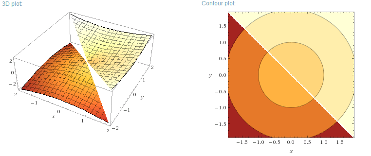
Flipping $s$ without introducing a discontinuity in the phase correction requires $|v|$ to be a whole number of half turns, since that's the only time when $e^{i \pi \theta} = e^{-i \pi \theta}$. But we need to flip $s$ for all $v$-vs-$-v$ pairs including ones that aren't half-turns, and we can swivel the axis around to make the flips meet, so... no matter what we do we're going to end up with a discontinuity in our phase correction angle. Something like this:
(Okay you got me, it doesn't have to be one discontinuity. It can be more than one, too.)
We can orient the plane where the discontinuity occurs so that you're unlikely to use rotation axies along it, but there's no way to avoid the fact that there is a plane-of-terribleness in the first place (... without changing to a different approach).
Note that, even if you avoid rotation axies along the bad plane, you'll still run into problems when combining multiple rotations. This is a consequence of wanting half turns to correspond to the Pauli matrices. There's no way to avoid accumulating a global phase factor via multiple rotations because, although rotating a half turn around the X then Y then Z axis gives you no net rotation, $\sigma_x \cdot \sigma_y \cdot \sigma_z = i I \neq I$.
So, although we've solved two flaws from the original mapping (720° turns and no way to get the Pauli matrices), we've introduced a discontinuity where the sign of the result switches as you swivel the rotation axis and we still have a multiple-rotations-can-accumulate-phase problem. Whether or not those flaws are preferable to the original flaws depends on the application.
Implementation
Here is python code implementing the final mapping from above:
# Warning: flawed; see below
def rotation_to_matrix(x=0, y=0, z=0):
    s = math.copysign(1, -11*x + -13*y + -17*z)  # phase correction discontinuity on an awkward plane
    theta = math.sqrt(x**2 + y**2 + z**2)
    v = x * np.mat([[0, 1], [1, 0]]) +\
        y * np.mat([[0, -1j], [1j, 0]]) +\
        z * np.mat([[1, 0], [0, -1]])

    ci = 1 + cmath.exp(1j * s * theta)
    cv = s * (1 - cmath.exp(1j * s * theta)) / theta  # Potential division by zero!

    return (np.identity(2) * ci - v * cv)/2
A notable problem in the above code is that we're dividing by the rotation angle in order to compute the unit vector along the axis of rotation. This will cause problems for small rotations. We could just have an "if rotation is small, default to the identity matrix" guard, but those are gross and generally poorly behaved. Instead, we're going to rewrite $\frac{1 - e^{i s \theta}}{\theta}$ so it doesn't involve a division.
To avoid the division, we're going to use the sinc function: $\mathrm{sinc}(x) = \frac{\sin x}{x}$. To get to that point we'll expand the $exp$ into trig functions, simplify, use the half-angle identities, and simplify:
$\frac{1 - e^{i s \theta}}{\theta}$
$= \frac{1 - (\cos(s \theta) + i \sin(s \theta))}{\theta}$
$= \frac{1 - \cos(\theta)}{\theta} - \frac{i s\sin(\theta)}{\theta}$
$= \frac{1 - (1 - 2 \sin^2 \frac{\theta}{2})}{\theta} - \frac{i s \sin \theta}{\theta}$
$= \frac{\sin^2 \frac{1}{2} \theta}{\frac{1}{2} \theta} - i \: s \: \frac{\sin{\theta}}{\theta}$
$= \sin \frac{\theta}{2} \mathrm{sinc} \frac{\theta}{2} - i \: s \: \mathrm{sinc} \: \theta$
Although sinc also has a division by zero, we can use the fact that $\sin x$ acts like $x$ near zero to cancel out the problem. As we get close to zero, the Taylor series $\sin x = x - \frac{x^3}{3!} + \frac{x^5}{5!} - ...$ divided by $x$ gives a good enough approximation $\frac{\sin x}{x} = 1 - \frac{x^2}{3!} + \frac{x^4}{5!} - ... \approx 1 - \frac{x^2}{6}$. We'll switch from directly computing $\frac{\sin x}{x}$ to using the approximation around the time where $1 + \frac{x^4}{120}$ starts getting rounded to $1$.
Given the stable sinc function, and the arbitrarily chosen plane-of-terribleness, we can write the continuous-near-half-turns-and-away-from-the-plane-of-terribleness rotation_to_matrix function:
import numpy as np
import cmath
import math


def rotation_to_matrix(x=0, y=0, z=0):
    """
    Returns a unitary matrix that corresponds, in a useful but not unique way, to a rotation around
    the axis <x, y, z> by sqrt(x^2 + y^2 + z^2) radians.
    """
    s = math.copysign(1, -11*x + -13*y + -17*z)  # phase correction discontinuity on an awkward plane
    theta = math.sqrt(x**2 + y**2 + z**2)
    v = x * np.mat([[0, 1], [1, 0]]) +\
        y * np.mat([[0, -1j], [1j, 0]]) +\
        z * np.mat([[1, 0], [0, -1]])

    ci = 1 + cmath.exp(1j * s * theta)
    cv = math.sin(theta/2) * sinc(theta/2) - 1j * s * sinc(theta)

    return (np.identity(2) * ci - s * v * cv)/2


def sinc(x):
    """
    Returns sin(x)/x, but computed in a way that doesn't explode when x is equal to or near zero.
    sinc(0) is 1.
    """
    if abs(x) < 0.0002:
        return 1 - x**2 / 6
    return math.sin(x) / x
And we can double-check that it's doing what we want by printing out a few test values:
np.set_printoptions(precision=5, suppress=True)

print "I", rotation_to_matrix()
print "I_2", rotation_to_matrix(x=2*math.pi)
print "X", rotation_to_matrix(x=math.pi)
print "Y", rotation_to_matrix(y=math.pi)
print "Z", rotation_to_matrix(z=math.pi)
print "H", rotation_to_matrix(x=math.pi / math.sqrt(2), z = math.pi / math.sqrt(2))
print "sqrt_1(X)", rotation_to_matrix(x=math.pi/2)
print "sqrt_2(X)", rotation_to_matrix(x=-math.pi/2)
Which prints:
I [[ 1.+0.j  0.+0.j]
 [ 0.+0.j  1.+0.j]]
I_2 [[ 1.+0.j  0.-0.j]
 [ 0.-0.j  1.+0.j]]
X [[ 0.-0.j  1.+0.j]
 [ 1.+0.j  0.-0.j]]
Y [[ 0.-0.j  0.-1.j]
 [-0.+1.j  0.-0.j]]
Z [[ 1.+0.j  0.+0.j]
 [ 0.+0.j -1.-0.j]]
H [[ 0.70711-0.j  0.70711+0.j]
 [ 0.70711+0.j -0.70711-0.j]]
sqrt_1(X) [[ 0.5-0.5j  0.5+0.5j]
 [ 0.5+0.5j  0.5-0.5j]]
sqrt_2(X) [[ 0.5+0.5j  0.5-0.5j]
 [ 0.5-0.5j  0.5+0.5j]]
Those values look good to me (modulo the rounding error introduced by the involvement of $\pi$ and $\sqrt{2}$). The half-turns along each axis give the corresponding Pauli matrix, rotating one full turn gets us back to the identity matrix, the quarter turns are square roots of the half turns, and we even manage to get the Hadamard matrix by rotating a half turn around the X+Z axis.
Summary
The common method for mapping rotations into unitary matrices is smooth, but can't generate the Pauli matrices and requires a 720° turn to get back to the starting point.
By applying a phase correction we can fix those issues, but we're forced to introduce a phase discontinuity w.r.t. the axis of rotation.
Update
Converting from rotations to operations is better understood in terms of matrix exponentation. See Using Eigendecomposition to Convert Rotations and Interpolate Operations.
